Linear Regression Analysis and Web Intelligence

This article looks at how to do linear regression analysis in Web Intelligence. Linear regression is a statistical technique for analysing data in order to obtain a measure of correlation between two variables where the relationship between the variables is expected to be linear.

Web Intelligence does not contain a full set of formula for calculating the typical linear regression coefficients and so we must use other formula to calculate these. This article looks at how to apply the Least Squares method for calculating linear regression in web Intelligence.

When to use Linear Regression Analysis

We use linear regression when we want to test a theory where as one variable changes then another variable will also change at a fixed rate. For example our theory could be that as we increase the number of users on our web server this will lead to an increase in memory usage. Here our statistical variables are number of users and memory.

Our theory about increasing the number of users leads to increased memory seems fairly obvious and you may think why would we need to do any further investigation however what we don’t know is by how much the memory increases per user or if in fact this increase is linear or exponential.

By linear we mean that as we increase the number of users we increase the memory by a fixed amount per user. For example every new user on the system would increase RAM by 2mb. Exponential growth would be where the amount the memory increase by would itself increase, for example the first dozen users or so increase memory by about 2mb each but the next 20 give an increase by about 4mb each and the next 20 again increase memory by about 8mb and so on.

Another example of where we can use regression analysis is in forecasting. If something is increasing or decreasing steadily over time then we can use this knowledge to make a forecast on a future value. Climate change is a topical example of this. Or if a company has increased it’s sales revenue by about $10,000 every month for the last 2 years then we can expect that it’ll carry on increasing by same amount for the next few months. Obviously as we go further into the future the less likely this will hold and this uncertainty can also be measured using linear regression techniques.

Charting

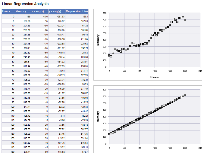
The easiest way to determine whether the relation between two variables is linear is to display the results on a chart. The example chart below shows measurements of number of users versus memory for a hypothetical web server.

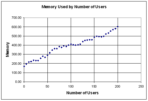
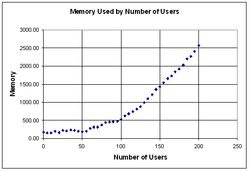
We can see that the points line up in a reasonable straight line and so this indicates that there is a good linear correlation between number of users a memory. By contrast this chart is an example of an exponential relation.

It is important to always chart your data sets as there can be some situations where even thought the analysis gives the same regression coefficients, the reality is very different. For examples of this see Anscombe’s Quartet.

Background to the Maths Involved

There are several different techniques for linear regression analysis but here we will look at using simple linear regression analysis using the “method of least squares”.

Here we fit a straight line through the of the data points that would provide the best fit to those points. This line is given by the equation,

where y and x are our variables e.g. number of users and memory consumption. b is known as the gradient and is the amount by which y increases for every increase in x, for example if every new user increases memory by 4mb then b here has value 4. a is known as the intercept and is the point where the straight line meets the y axis. In our example this would be the minimum amount of RAM used by the web server when there are no users on the system.

As well as calculating the two values a (intercept) and b (gradient) we also want to calculate the correlation coefficient (denoted by r) which is a measure of how well the points fit to the straight line. This is a value between 0 and 1 where a result of 0.5 or below would mean that there is little or no linear relationship while values above 0.8 would mean that there is a strong linear relationship.

For examples of different distributions and their r value see the examples in this topic from Wolfram. The correlation coefficient is also known as the product-moment coefficient of correlation or Pearson’s correlation. It is sometimes also expressed as a r-squared.

Gradient

We begin by calculating the gradient b. This is given by the formula,

which is the covariance in x and y divided by the variance in x. Covariance in x,y is given by the following formula,

and variance in x is given by

Intercept

Once we have found b we can then calculate the intercept (a) by,

That gives us the values we need for our straight line equation.

Correlation Coefficient

To calculate our correlation coefficient we use,

r = cov(x,y) / sqrt [ var(x) * var(y) ]

Correlation coefficient r equals covariance in x y divided by the square root of variance in x by the variance in y

Linear Regression Analysis in Web Intelligence

We will use a worked example to look at how we calculate the three coefficients a, b and r mentioned above. Our example is to look at number of users accessing a web server compared to system RAM. We will use Web Intelligence Rich Client and a set of data from a flat text file and this file can be downloaded from this link User Memory Test Data File.

It is easier to do this if we built up the formula in stages. First we begin by importing our data into a table where the two columns are our two variables. We duplicate this table and turn the second instance to a chart and confirm that our data set looks like a good candidate for linear regression.

Note, this article uses Web Intelligence XI 3.1 but the calculations may work in previous versions.

Create New Web Intelligence Document

First we create a new document and import our data

1. Create a new document using Web Intelligence Rich Client.
2. Browse for more Data Sources and select Other data source, Text and Excel Files
3. Browse to the text file you downloaded above. Make sure Tabulation is selected as format and click next
4. In the Create Query dialog check that both objects are Measures and click Run Query
5. The table will be displaying a single row which is the sum of all values. To see each row select the table, click Properties tab and under Display section and check on the option “Avoid duplicate row aggregation”
6. Also at this stage select display table footer as we’ll need to use this later.
7. Create a duplicate of the table and place to the right of the table,
8. Select the second table, right click and select Turn To
9. Select XY Scatter graph (under Radar Tab). Format the graph as required. Your document should look like the following,

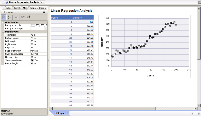
We can see from the chart that we have a reasonably good straight line so it make sense that we can do our linear regression analysis

The scatter chart in Web Intelligence is limited in it’s functionality and formatting options. By default it marks each data point in a different colour which doesn’t makes sense, nor does it give you the option to use a line rather than markers. Also unlike Excel there’s no option to add a trend line to the chart.

Covariance

First of all we want to calculate the covariance in the data and we’ll use this in the numerator (top half) of our regression formula for the gradient. We will build this formula in Web Intelligence in stages.

1. 1. Add a two new empty columns to the right hand side of the table.
   2. Label one “x–avg(x)” and the other “y–avg(y)”
   3. In the x-avg(x) column enter the formula,

=[Users]-Average([Users])

This should result in zeroes for the whole column. What is happening here is that the function Average([Users]) is only calculating the average for a single row which is going to be just the value of [Users]. What we need is for the Average function to calculate the average for the whole table. We do this using calculation contexts.

1. 1. Update our formula to,

=[Users]-( Average([Users]) In Block )

1. 1. And similar formula for memory,

=[Memory]-( Average([Memory]) In Block)

1. 1. Navigate down to the report footer and add “cov(x,y)” in x-avg(x) column
   2. and add the following formula next to this in the y-avg(y) column

=Sum( ([Users] -(Average([Users])  In Block)) *
      ([Memory]-(Average([Memory]) In Block)) ) In Block /
 ( Count([Users]) In Block )

You should get a value of 10,210.6. To make further calculations easier we will convert this formula to a Web Intelligence variable.

1. Display the formula tool bar
2. Select the cell that contains the above formula and click the icon on the formula toolbar to create a new variable
3. Give the new variable the name “Covariance”

Variance

Web Intelligence does have a built in formula for variance and so we can just use this,

1. 1. Add a new row to the footer, add “var(x)” in the x-avg(x) column and add the following formula in the adjacent cell in the y-avg(y) column,

=VarP([Users])

This should give a value of 3,500

Gradient (b)

To calculate the gradient for our straight line we then divide the covariance by the variance

1. 1. Add a third footer row and enter “gradient” under the x-avg(x) column and add the following formula in the adjacent cell,

=[Covariance] / VarP([Users]) In Block

This should give you a value of 2.92.

1. Also create this as a new variable called Gradient

This means that each new user on system will increase RAM by on average 2.92 MB. So if we add 500 users to the system we can expect RAM to be 1,460 MB plus whatever the base level was. The base level is how much RAM the system uses before we add any users. We determine this by calculating the intercept coefficient.

Intercept (a)

To calculate the intercept we use the gradient and the average values of x and y,

1. 1. Add a new footer row with “intercept” in the x-avg(x) column and the following formula in the adjacent cell,

=(Average([Memory]) In Block) –
 ( [Gradient] * Average([Users]) In Block )

This should give a value of 138.10

1. And create this as a new variable called Intercept.

Correlation Coefficient (r)

The correlation coefficient is a measure of how well the data fits to a straight line.

1. 1. Add a new footer row and enter “r” in the x-avg(x) column and the following formula in the adjacent cell,

=[Covariance] / Sqrt( VarP([Users])*VarP([Memory]) )

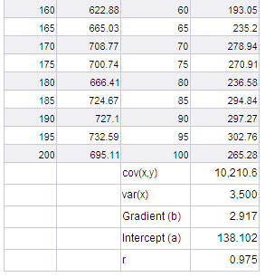
And here we should get a value of 0.975 which indicates that we have a pretty good linear correlation between number of users and increase in memory.

Our table should look like the following,

Add Our Straight Line to Chart

Now that we’ve calculated our gradient and intercept we can use these to generate a new set of data which we can plot as a straight line to our chart. Unfortunately we can’t add a 2nd data set to a scatter chart in Web Intelligence. We can add additional data sets to a standard line chart but here we need to use the scatter chart as our x-axis variable may not be at a regular intervals.

In our example above the x-axis variable – number of users – does increment by a regular amount and so we could use a line chart to display the straight line. What we can do though is to create a new chart that just displays our straight line,

1. 1. Add a new column to the table, label this column regression line
   2. Enter the following formula (which is the equation of our straight line ) in the body cells of the column

=[Gradient] * [Users] + [Intercept]

1. Duplicate this table and position new table below existing chart
2. Remove all columns except Users and our new Regression Line column
3. Right click, Turn To and select scatter chart again and we should now get a nice straight line chart,

Summary

So to summarise the steps above,

1. 1. Create a new variable called Covariance with the following formula,

=Sum( ([x]-(Average([x]) In Block)) *
      ([y]-(Average([y]) In Block))) In Block / Count([x])

1. 1. Create and display a new variable called Gradient with the following formula,

=[Covariance] / VarP([X]) In Block

1. 1. Create and display a new variable called intercept,

=(Average([Memory]) In Block) –
 ( [Gradient] * Average([Users]) In Block )

1. 1. Calculate and display the correlation coefficient,

=[Covariance] / Sqrt( VarP([x])*VarP([y]) )

Conclusion

Unfortunately built in functionality for statistical analysis is one area where Web Intelligence is weaker than Excel. Even for basic analysis such as linear regression we find that Web Intelligence has some but not all statistical formula we would like. However as we seen from above it is always possible to build up the required calculations by using other built in functions.

Hopefully future releases of Web Intelligence will contain more statistical analysis functions and improved charting!

References and Further Reading

http://en.wikipedia.org/wiki/Linear_regression

http://en.wikipedia.org/wiki/Anscombe%27s_quartet

http://en.wikipedia.org/wiki/Forecasting

http://phoenix.phys.clemson.edu/tutorials/excel/regression.html

http://serc.carleton.edu/introgeo/teachingwdata/StatRegression.html

http://www.statistics-help-online.com/node51.html

Weisstein, Eric W. “Least Squares Fitting” from MathWorld – A Wolfram Web Resource.

Weisstein, Eric W. “Correlation Coefficient” from MathWorld – A Wolfram Web Resource.