Introduction
A moving average is a simple technique for smoothing random data. Most often we find moving averages to analyse movement of stock prices but we also see them in other areas of business and data analysis.
This is the first part of a series of two articles. This article discusses what are moving averages and how they are calculated. The second part then looks at how to implement moving average calculations in SAP BusinessObjects Web Intelligence.
If you already understand moving averages you can skip to the second article on how to implement in Web Intelligence.
What Are Moving Averages
A moving average analyses a set of data points by calculating an average over a smaller set of recent data points. For example when analysing stock price over a year we can generate a moving average that for a given day is the average of the last 15 days. Figure 1 below is an example of a simple moving average generated with Google Finance. This chart displays Google’s stock price over the last year and the red line is a moving average with a period of 15 days.

We can see from the above example that the moving average (red line) smooths out the fluctuating stock price. A feature of a moving average is that it lags behind the original curve. This is because at each data point it takes an average of a set of previous data points. For a further discussion of how moving averages are used in finance see Moving Averages at StockCharts.com.
The objective of using a moving average is to reduce short term fluctuations and to highlight longer term trends. There are several different types of moving average and below we’ll look at how to calculate the more common examples. After this we’ll then look at how to implement these calculations in Web Intelligence.
Simple Moving Average
A Simple Moving Average (SMA) as it’s name suggests is the easiest moving average to calculate. For each data point we calculate the average over a fixed number of preceding data points. The table below illustrates such a calculation where we are using an SMA of period 3.
| Stock Price | Calculation | Result |
|---|---|---|
| 616.26 | ||
| 621.63 | ||
| 637.77 | ( 616.26 + 621.63 + 637.77 ) / 3 | 625.22 |
| 632.06 | ( 621.63 + 637.77 + 632.06 ) / 3 | 630.49 |
| 628.17 | ( 637.77 + 632.06 + 628.17 ) / 3 | 632.67 |
| 625.27 | ( 632.06 + 628.17 + 625.27 ) / 3 | 628.50 |
As our the period of our moving average data set is 3 we don’t calculate the first two data points. Then for each data point we calculate the average over the last three data points including the current data point. Since when calculating our average the latest value is added to the sum and the first value drops out we can simplify our calculation to,
SMA = SMA(previous) – (p1 / N) + (pN / N)
Where SMA(previous) is the result we previously calculated, N is the size of the moving average data set, p1 is the first value in our set and pN is the last value of the set.
A draw back of an SMA is that it treats all previous data points in the moving average set equally and so we can find that older data points can negatively influence the calculation. To address this we can use weighted or exponential moving averages.
Weighted Moving Average
A weighted moving average (WMA) applies weights to the data points in the moving average set such that more recent data points have more significance to the overall result. There are several ways we can apply weights and the simplest is to use a decreasing set of weights, for example, if we have a moving average data set of 6 data points then our weights are 6,5,4,3,2,1 applied from the most recent data to the earliest. Our calculation is a bit more complex and for a moving average data set of size 6 it is,
WMA = ( 6*p6 + 5*p5 + 4*p4 + 3*p3 + 2*p2 + p1 ) / 6*(6+1)/2
So here p6 is our current value and we multiply this by 6, we then add 5 times the previous value, 4 times the value before that and so on. We then divide this by 6*(6+1)/2. This is the calculation for a triangular number and Wikipedia has an explanation of how this is derived.
The table below illustrates the calculation of a WMA of period 3 for the same data set we used in the SMA example above.
| Stock Price | Calculation | Result |
|---|---|---|
| 616.26 | ||
| 621.63 | ||
| 637.77 | ( 3*616.26 + 2*621.63 + 637.77 ) / 3*(3+1)/2 | 628.81 |
| 632.06 | ( 3*621.63 + 2*637.77 + 632.06 ) / 3*(3+1)/2 | 632.23 |
| 628.17 | ( 3*637.77 + 2*632.06 + 628.17 ) / 3*(3+1)/2 | 631.07 |
| 625.27 | ( 3*632.06 + 2*628.17 + 625.27 ) / 3*(3+1)/2 | 627.37 |
Exponential Moving Average
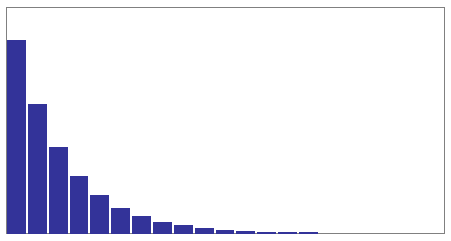
An exponential moving average (EMA) uses an exponentially decreasing set of weights. In the WMA above our weights decreased linearly, an exponentially decreasing set of weights reduce rapidly at first and then tails off. If we produce a graph of these weights it would look something like figure 2 below.
An EMA provides more weight to recent values than a WMA and it also has the further advantage of being more easily calculated. To calculate an EMA we take the previous EMA value and add the difference between the current data point value and the previous EMA multiplied by a constant ‘alpha’,
EMA = EMA(previous) + alpha * [pN – EMA(previous)]
The constant alpha represents the scale of weighting decrease and is a value between 0 to 1. Changing this value changes the amount of overall smoothing where values close to zero apply a high degree of smoothing and values nearer 1 produce less. The figure below uses the same data points but display an EMA of value 0.7 and 0.1.

In our calculations we only apply the EMA from the 3rd data point onwards for the first data point it is customary to set this to 0 or no value and for the 2nd data point we set the value to be equal to the value of the 2nd data point.
The table below is the calculation of EMA for our example data set using an alpha value of 0.4
| Stock Price | Calculation | Result |
|---|---|---|
| 616.26 | ||
| 621.63 | 621.63 | 621.63 |
| 637.77 | 621.63 + 0.4 * (637.77 – 621.63) | 628.09 |
| 632.06 | 628.09 + 0.4 * (632.06 – 628.09) | 629.68 |
| 628.17 | 629.68 + 0.4 * (628.17 – 629.68) | 629.07 |
| 625.27 | 629.07 + 0.4 * (625.27 – 629.07) | 627.55 |
OK now that we know about moving averages the next article looks at how to implement these 3 types in Web Intelligence.
